The Math Behind Keras 3 Optimizers: Deep Understanding and Application

Introduction

Optimizers are an essential part of everyone working in machine learning.

We all know optimizers determine how the model will converge the loss function during gradient descent. Thus, using the right optimizer can boost the performance and the efficiency of model training.

Besides classic papers, many books explain the principles behind optimizers in simple terms.

However, I recently found that the performance of Keras 3 optimizers doesn't quite match the mathematical algorithms described in these books, which made me a bit anxious. I worried about misunderstanding something or about updates in the latest version of Keras affecting the optimizers.

So, I reviewed the source code of several common optimizers in Keras 3 and revisited their use cases. Now, I want to share this knowledge to save you time and help you master Keras 3 optimizers more quickly.

If you're not very familiar with the latest changes in Keras 3, here's a quick rundown: Keras 3 integrates TensorFlow, PyTorch, and JAX, allowing us to use cutting-edge deep learning frameworks easily through Keras APIs.

Keras 3.0 Tutorial: End-to-End Deep Learning Project Guide

Implement an encoder-decoder recurrent network from scratch

Data Leads FuturePeng Qian

Preparation

Some utility methods

I plan to show you through some charts how these optimizers affect the convergence of loss functions.

Before starting, I need to prepare some utility methods for creating these charts.

First, I'll use sklearn to generate a virtual dataset for a classification task:

from sklearn.datasets import make_moons
X, y = make_moons(n_samples=300, noise=0.1, random_state=42)

Since the dataset is quite simple, I plan to build a basic multilayer perceptron model with three hidden layers and a dual-node output layer:

from keras import layers, utils, ops
import keras

def build_model(input_shape: tuple):
    inputs = layers.Input(shape=input_shape)
    x = layers.Dense(12, activation='relu')(inputs)
    x = layers.Dense(13, activation='relu')(x)
    x = layers.Dense(13, activation='relu')(x)
    outputs = layers.Dense(2, activation='softmax')(x)
    return keras.Model(inputs=inputs, outputs=outputs)

Finally, our utility method will evaluate how different optimizers affect model loss convergence. It also takes a parameter for epochs to highlight details of some optimizers.

This method will also use the matplotlib library to plot the model loss convergence curves, making the assessment more visual:

def fit_show_model(optimizer: keras.optimizers.Optimizer,
                      epochs: int = 800
                    ):
    my_model = build_model(input_shape=(2,))
    my_model.compile(optimizer=optimizer, 
                     loss='sparse_categorical_crossentropy', 
                     metrics=['accuracy'])
    history = my_model.fit(X, y, batch_size=32, epochs=epochs, verbose=0)
    loss=history.history['loss']
    _, ax = plt.subplots(figsize=(5, 3))
    ax.plot(range(len(loss)), loss, 'b')
    ax.set(
        xlabel="Epoch",
        ylabel="Loss"
    )
    plt.show()

Variable abbreviations

Since this article is full of mathematical expressions, I plan to abbreviate some common variables to make these expressions clearer. For example:

• lr stands for learning_rate.
• g represents the gradient at the current node.
• e is epsilon, a very small number added to the denominator to prevent it from being zero.
• sqrt refers to np.sqrt or ops.sqrt, which is used to take the square root of an expression.

After these preparations, I will start explaining each optimizer.

Detailed Explanation of Common Optimizers

SGD

Also known as Stochastic Gradient Descent, it's almost everyone's first encounter with an optimizer.

Its principle is simple: randomly select a small batch of data samples, calculate the gradient at each node, and then update the weight of the current node using the learning rate.

In Keras 3, its mathematical expression is as follows:

w = w - lr * g

We can use SGD as a baseline to visually compare the effects of other optimizers:

fit_show_model(optimizer=keras.optimizers.SGD(learning_rate=0.01))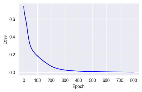

SGD's biggest drawback is that its learning rate is fixed at every point on the curve, leading to quick weight changes on steep slopes and slow changes on flat ones. This makes it easy to get stuck in local minima (a phenomenon well-documented elsewhere, so I won't repeat it here).

How can we avoid getting stuck? Just like helping a car out of the mud, we can give momentum to the weight changes to push it forward, solving this problem.

The mathematical expression with momentum is shown below:

m = momentum * m - lr * g

You can see that momentum speeds up loss convergence:

fit_show_model(optimizer=keras.optimizers.SGD(learning_rate=0.01, 
                                              momentum=0.9))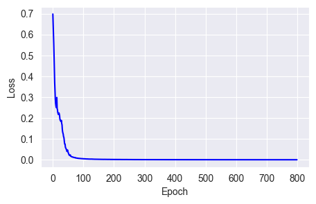

As mentioned before, since SGD's learning rate is fixed, we need to set a reasonable learning rate. If it's too high, the weight will oscillate back and forth across the valley. If it's too low, the weight will take longer to find the valley, and more likely to get stuck.

To address this, besides using momentum, we can also predict the next direction of the weight change and add this prediction to the current weight. This method is called the Nesterov method. Its mathematical expression is as follows:

m = momentum * m - lr * g
w = w + (momentum * m -lr * g)

fit_show_model(optimizer=keras.optimizers.SGD(learning_rate=0.01,
                                              momentum=0.9,
                                              nesterov=True))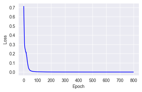

You can see that in Keras 3, using the Nesterov method requires setting the momentum parameter first; otherwise, we can't predict the direction of the next weight change.

Adagrad

After discussing algorithms related to stochastic gradient descent, let's talk about optimizers related to adaptive algorithms. The simplest one is Adagrad.

The core idea of adaptive algorithms is to dynamically adjust the learning rate as training progresses.

Based on this idea, Adagrad adjusts the learning rate by accumulating the sum of the squares of the gradients from historical iterations and dividing the learning rate by this sum. In Keras 3, Adagrad's mathematical expression is as follows:

accumulator = accumulator + g**2
w = w - (lr * g) / sqrt(accumulator + e)

fit_show_model(optimizer=keras.optimizers.Adagrad(learning_rate=0.01))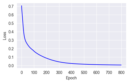

From the chart, we can see that Adagrad does not converge losses very quickly, even slower than the default SGD algorithm, because the learning rate decreases as training progresses.

RMSprop

To address the issue of Adagrad decreasing the learning rate too much, Hinton proposed an improved algorithm in 2012. This algorithm doesn't simply add up the squares of the gradients; it assigns a weight to the square of each gradient, giving more weight to recent iterations. The rest of the calculation is similar to Adagrad.

v = rho * v + (1 - rho) * g**2
w = w - lr * g / sqrt(v + e)

fit_show_model(optimizer=keras.optimizers.RMSprop(learning_rate=0.01),
               epochs=100)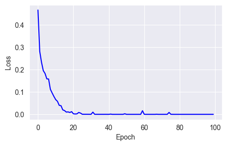

As you can see, although loss convergence isn't very stable, it reaches near zero around 40 epochs, much faster than Adagrad and SGD.

In Keras 3, RMSprop also supports setting momentum and centered parameters. Momentum adds momentum to the weight changes, and if the centered parameter is set, the optimizer doesn't directly use the accumulated square of the gradients but makes a correction using the moving average of the gradients. The expression is as follows:

v = rho * v + (1 - rho) * g**2
average_grad = rho * average_grad + (1 - rho) * g
m = momentum * m + (lr * g) / sqrt(v - average_grad**2 + e)
w = w - m

fit_show_model(optimizer=keras.optimizers.RMSprop(learning_rate=0.01,
                                                  momentum=0.9,
                                                  centered=True),
               epochs=100)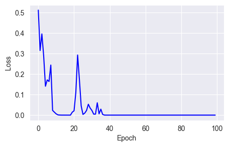

You can see that using the momentum and centered parameters, RMSprop converges losses faster but still has stability issues.

Adam

Let's talk about the Adam optimizer. Unlike the previous two algorithms, Adam not only uses the accumulated square of the gradients but also the first moment of the gradients. So, Adam has two extra hyperparameters: beta_1 and beta_2.

In Keras 3, Adam has evolved further. Now, it adjusts beta_1 and beta_2 exponentially based on the current step of the iteration, affecting the size of the learning rate. This evolution makes the Adam optimizer very suitable for time-sensitive scenarios like speech recognition:

t = 0 # current iteration 
local_step = t + 1 
beta_1_power = power(beta_1, local_step) 
beta_2_power = power(beta_2, local_step) 
alpha = lr * sqrt(1 - beta_2_power) / (1 - beta_1_power) 
m = m + (1 - beta_1) * (g - m) 
v = v + (1 - beta_2) * (g**2 - v) 
w = w - (alpha * m) / (sqrt(v) + e)

fit_show_model(optimizer=keras.optimizers.Adam(learning_rate=0.01),
               epochs=100)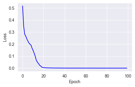

From the chart, you can see that the Adam optimizer converges losses very quickly and smoothly, reaching near zero by the 20th epoch.

AdamW

In Keras 3, there is also an optimizer called AdamW, which, as the name suggests, is similar to Adam but adjusts the weights with a constant decay amount through the weight_decay parameter.

w = w - weight_decay * lr * w

fit_show_model(optimizer=keras.optimizers.AdamW(learning_rate=0.01,
                                                weight_decay=0.01),
               epochs=100)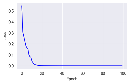

From the source code, it's clear that the AdamW optimizer is actually calling the Adam optimizer and assigning a value to the weight_decay parameter.

Nadam

Then there is the Nadam optimizer, which, as the name suggests, is a variant of the Adam optimizer.

In Keras 3, it incorporates the idea of Nesterov, not only focusing on the current iteration step but also on the impact of the next step. Then it combines these two effects on the beta_1 and beta_2 parameters.

So, of all the optimizers, Nadam's algorithm is the most complex:

t = 0 
decay = 0.96 
local_step = t + 1 
next_step = t + 2

u_t = beta_1 * (1.0 - 0.5 * power(decay, local_step)) 
u_t_1 = beta_2 * (1.0 - 0.5 * power(decay, next_step)) 
u_product_t = u_product_t * beta_1 * (1.0 - 0.5 * power(decay, local_step))

u_product_t_1 = u_product_t * u_t_1

beta_2_power = power(beta_2, local_step)
m = m + (1 - beta_1) * (g - m) 
v = v + (1 - beta_2) * (g**2 - v)
m_hat = u_t_1 * m / (1 - u_product_t_1) + ((1 - u_t) * g) / (1 - u_product_t) 
v_hat = v / (1 - beta_2_power)

w = w - (lr * m_hat) / (sqrt(v_hat) + epsilon)

fit_show_model(optimizer=keras.optimizers.Nadam(learning_rate=0.01),
               epochs=100)

However, for some simple classification tasks, the improvement from Nadam is not much.

Lion

Finally, let me mention the Lion optimizer, a new implementation proposed by Chen et al., 2023. This optimizer's biggest feature is that it doesn't calculate accumulations, so it uses less memory. It also doesn't calculate the second moment, so it's less complex.

It simply calculates a sign based on the current gradient and lets the weight and learning rate change according to this sign:

w = w - lr * sign(beta_1 * m + (1 - beta_1) * g)
m = beta_2 * m + (1 - beta_2) * g

fit_show_model(optimizer=keras.optimizers.Lion(learning_rate=0.001),
               epochs=100)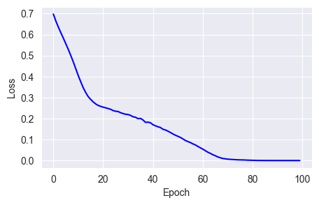

You can see that the performance of this optimizer isn't as good as the Adam series, probably the price paid for saving resources.

Conclusion

As mentioned at the beginning of the article, optimizers, as one of the most critical parts of deep learning, are skills that every practitioner needs to master and apply.

Also, with technological advancements, the implementation of optimizers within the latest deep learning frameworks is continuously evolving in terms of computational efficiency and application scenarios.

This article introduced the mathematical implementation of several common optimizers in Keras 3.

If you're still confused about how to use the optimizers in Keras 3, I suggest starting with Adam. After achieving good results, you can choose a more suitable optimizer based on specific scenarios.

What else would you like to know about Keras 3? Feel free to leave comments and discuss. See you next time.